Who cares about stopping rules?

Can you bias a coin?

Challenge: Take a coin out of your pocket. Unless you own some exotic currency, your coin is fair: it’s equally likely to land heads as tails when flipped. Your challenge is to modify the coin somehow—by sticking putty on one side, say, or bending it—so that the coin becomes biased, one way or the other. Try it!

How should you check whether you managed to bias your coin? Well, it will surely involve flipping it repeatedly and observing the outcome, a sequence of h‘s and t‘s. That much is obvious. But what’s not obvious is where to go from there. For one thing, any outcome whatsoever is consistent both with the coin’s being fair and with its being biased. (After all, it’s possible, even if not probable, for a fair coin to land heads every time you flip it, or a biased coin to land heads just as often as tails.) So no outcome is decisive. Worse than that, on the assumption that the coin is fair any two sequences of h‘s and t‘s (of the same length) are equally likely. So how could one sequence tell against the coin’s being fair and another not?

We face problems like these whenever we need to evaluate a probabilistic hypothesis. Since probabilistic hypotheses come up everywhere—from polling to genetics, from climate change to drug testing, from sports analytics to statistical mechanics—the problems are pressing.

Enter significance testing, an extremely popular method of evaluating probabilistic hypotheses. Scientific journals are littered with reports of significance tests; almost any introductory statistics course will teach the method. It’s so popular that the jargon of significance testing—null hypothesis, $p$-value, statistical significance—has entered common parlance.

As common as it is, significance testing is controversial. Some people argue that the method needs to be used with caution; a plug-and-play approach will lead us astray. Others go further, arguing that significance tests are bunk: that the result of a significance test is no guide to the truth of the hypothesis being tested. Colin Howson and Peter Urbach put the claim forcefully:

[Significance tests] are advocated in hundreds of books that are recommended texts in thousands of institutions of higher education, and required reading for hundreds of thousands of students. [Yet] judgments of ‘significance’ and ‘non-significance’ carry no inductive meaning at all. Therefore they cannot be used to arbitrate between rival theories or to determine practical policy.

(Howson and Urbach, 2006: 181–2)

Strong stuff! This post focuses on one objection to significance testing: that significance tests are sensitive to the stopping rule.

First, we’ll see how significance tests work. Then we’ll show that they are sensitive to the stopping rule. And finally we’ll look at some of the back and forth on whether sensitivity to the stopping rule is a problem.

Primer on probability

This section reviews some facts about probability needed later. We’ll work up to solving the following problem: What’s the probability of getting $m$ heads in $n$ flips of a coin, where the probability of heads on any given flip is $q$? If you already know what this is, jump to the next section; else, expand the material below.

Suppose we’re flipping a coin. We’ll make two assumptions. First, that the coin lands heads or tails on each flip (no landing on its side or spontaneously combusting). Second, that the probability of landing heads on any flip is independent of the pattern of prior flips: some constant number $q$. The first assumption isn’t really restrictive—after all, we can always discard any flip where the coin does something exotic and flip again. The second assumption is substantive; but it’s well-confirmed by theory and practice.

Given these assumptions, what’s the chance of getting $m$ heads if we flip the coin $n$ times? We need three facts about probability to answer this question:

Fact 1: The probability of independent events co-occurring is the product of the probabilities of the individual events. For example, if I flip the coin twice, and there’s a 50% chance of getting heads on each flip, then there’s a 25% (= 50% $\cdot$ 50%) chance of getting two heads.

Fact 2: The probability of one of several distinct events occurring is the sum of the probabilities of the individual events. For example, if I flip the coin twice, and there’s a 25% chance of getting two heads and a 25% chance of getting two tails, then there’s a 50% (= 25% + 25%) chance of getting either two heads or two tails.

Fact 3: The probability of an event $not$ $occurring$ is 1 minus the probability of the event occurring.

To get exactly $m$ heads in $n$ coin flips, I have to get some particular sequence of results that has a total of $m$ heads (and thus $n-m$ tails). What’s the chance of getting that particular sequence? By Fact 1, it’s the product of the probabilities of each result in the sequence. The probability of getting heads is $q$; there are $m$ of these. By Fact 3, the probability of getting tails is $1-q$; there are $n-m$ of these. So the probability of the particular sequence is the result of multiplying $q$ a total of $m$ times by $(1-q)$ a total of $n-m$ times: this is $q^m (1-q)^{n-m}$.

But there are lots of different sequences of $n$ coin flips that result in $m$ heads. Let’s call the number of such sequences $K$. Once we know $K$, we’re done: by Fact 2, the total probability of getting any one of the $K$ sequences with exactly $m$ heads is the sum of the probabilities of the individual sequences of this sort; each of these has the same probability, which we calculated in the preceding paragraph, of $q^m (1-q)^{n-m}$. So the total probability is just this added to itself $K$ times, which is just $K q^m (1-q)^{n-m}$.

So what’s $K$, the number of different possible sequences of $n$ coin flips that have exactly $m$ heads in them? Well, it’s equal to the number of different ways to pick $m$ objects out of a group of $n$ objects. To see this, note that we can represent any sequence of flips as a way of filling in a sequence of $n$ blanks _ _ _ … _ with ‘h‘ and ‘t‘ (in the obvious correspondence): every way I can fill in the blanks with ‘h‘s and ‘t‘s represents a unique way the flip could go, and every possible sequence of flips has such a representation. If I’m going to have a representation of exactly $m$ heads, I have to fill in exactly $m$ of these blanks with ‘h‘. I can pick any $m$ of the blanks to fill in with ‘h‘, but once I pick those, the rest have to be ‘t‘. So the number of possible $m$-heads flips is exactly the same as the number of possible choices of $m$ blanks out of $n$, or, more generally, the number of possible ways to pick $m$ objects from a collection of $n$ objects. Because this situation is common, this number gets a special symbol: $n \choose m$, pronounced ‘n choose m.’

OK, so what’s $n \choose m$? That is to say, how many different ways are there to pick $m$ objects out of a bucket of $n$ total objects? Well, when I’m just starting out, I haven’t chosen any; there are $n$ objects in the bucket, and so there are $n$ possible choices I can make for my first object. Now there are $n-1$ objects left in the bucket; so I have $n-1$ choices for my second object. And so on until I get to object number $m$, at which point there are $n-m+1$ objects left in the bucket. So the number of ways to choose $m$ objects out of $n$ objects, *in order*, is $n (n-1) (n-2) \cdots (n-m+1)$. But this isn’t quite the answer to our question, because what we care about is the number of ways of picking $m$ objects, not the number of ways of picking $m$ objects in order: getting the same objects in a different order doesn’t count as a different way of picking $m$ objects. So if $n (n-1) (n-2) \cdots (n-m+1)$ is the number of ways of picking $m$ objects, paying attention to the order, we need to divide by the number of ways of ordering $m$ objects to get the number of ways of picking $m$ objects, disregarding order. The number of ways of ordering $m$ objects, though, is given by exactly the reasoning we just went through: it’s the number of ways of picking $m$ objects in order from a group of $m$ objects, or $m (m-1) (m-2) \cdots (m-m+1 = 1)$, or, in other words, $m!$. Adding this reduction factor gives us the formula we want:

$${n \choose m} = \frac{n (n-1) \cdots (n-m+1)}{m!}$$

Finally, we can notice that $n (n-1) (n-2) \cdots (n-m+1)$ equals

$$\frac{n (n-1) (n-2) \cdots (n-m+1) (n-m) (n-m -1) \cdots 1}{(n-m)(n-m-1)\cdots 1}$$

which can be rewritten more briefly as

$$\frac{n!}{(n-m)!}$$

giving us the usual formula ${n \choose m} = \frac{n!}{m! (n-m)!}$

So putting it all together, the probability of getting $m$ heads out of $n$ flips, where the chance of any individual flip landing heads is $q$, is just ${n \choose m} q^m (1-q)^{n-m}.$

When I flip a coin $n$ times where the chance of any individual flip landing heads is $q$, how many heads will I get? Well, it depends. I might get 0 h‘s, or 1, or 2 , or …, or $n$. Which number I actually get is a chancy matter. For that reason, the number of heads is known as a *random variable*; the possible values of this random variable are 0, 1, …, 20. While each of these is a possible value, some values are more likely than others. The formula we just derived gives the probability of each. It’s known as the *distribution* of the number of heads. And because this—or close variants of it—is such a common situation, this is one of the probability distributions that gets a special name: it’s called the *binomial distribution*.

Here’s what the distribution looks like, in numbers, for a fair coin ($q=0.5$) flipped 10 times.

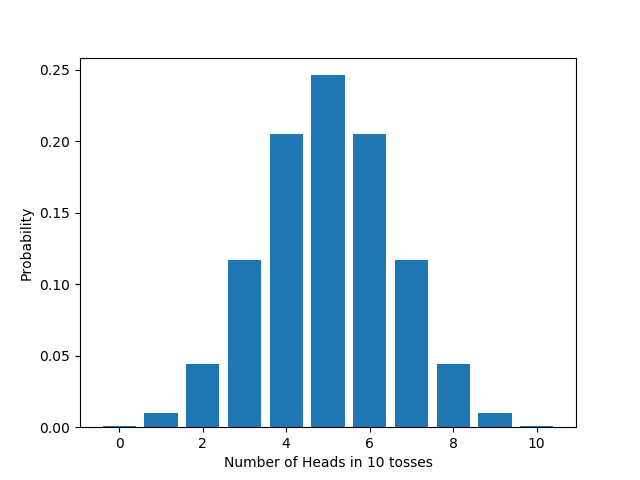
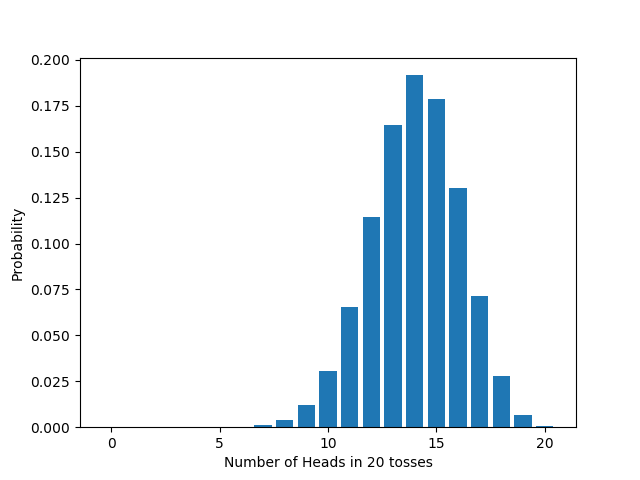
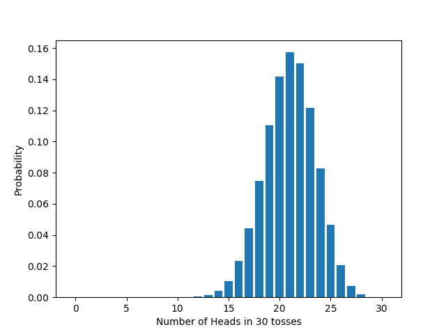
If we vary $n$, the number of times we flip the coin, the distribution changes too, in accord with the formula we derived above. For example:

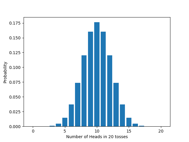
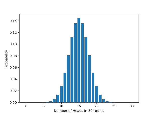
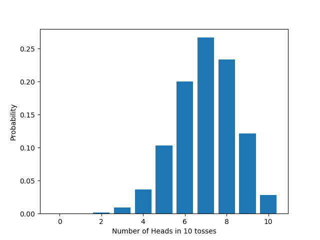
And if we take a biased coin ($q=0.7$), again the distribution changes, in accord with the formula above. For example:

How significance tests work

A significance test is a method of evaluating a probabilistic hypothesis. How do significance tests work? The procedure itself is quite simple, but the motivation for the procedure is subtle. So let’s build up to it in stages, to understand why it works the way it does.

Building up to a significance test

Remember the coin you modified earlier. We want to evaluate the hypothesis that the coin is fair. Suppose we flip it some number of times, and see that there are many more heads than tails. Does this give us reason to think it’s biased?

This is a tricky question because, as pointed out earlier, a fair coin can produce any outcome—and so can a biased coin (as long as there’s some non-zero chance of it landing heads and tails). In other words, if you flip your coin repeatedly and look at the resulting sequence, you can’t tell for sure whether your coin is fair or biased. To take an extreme case: it’s possible to flip a fair coin 1000 times and get heads every time. That’s the nature of chance.

Still, even though your coin—fair or biased—can produce any outcome, some outcomes are more likely than others, depending on the bias of the coin. Take the extreme case above: the probability of flipping a fair coin 1000 times and getting heads every time is $0.5^{1000}$. That’s small. In decimals, it’s about

0.0000000000000000000000000000000000000000000000000000000000000000000000000000000000000000000000000000000000000000000000000000000000000000000000000000000000000000000000000000000000000000000000000000000000000000000000000000000000000000000000000000000000000000000000000000000000000000000000000000000000000093326

So if we flip a coin 1000 times and get heads every single time, we might think that the sheer improbability of getting this sequence for a fair coin gives us very good reason to think that the coin isn’t fair. In other words, we might think that if our result is very improbable on the assumption that the coin is fair, we should reject that assumption.

But wait a second. There’s a big problem with this line of thought. Suppose your coin is fair, and suppose you flip it 1000 times and get not a sequence of 1000 heads, but some other sequence of heads and tails, say:

TTHHHTHHTHHTHTHHTHHHHHTT … HHTTTTTTHTHTTTHTHTHHHTHT

What’s the probability of getting this sequence, assuming the coin is fair? Well, it’s $0.5^{1000}$—exactly the same as the chance of getting 1000 heads. A fair coin has an equal chance of getting any particular sequence—the chance of getting any one of them is extraordinarily tiny. But surely not every outcome gives us reason to think the coin is biased.

So the reasoning we just went through can’t be right. We need something stronger than just the claim that our particular result was improbable. But we can modify the reasoning in a way that gets around this worry, by looking not at the result itself, but at properties of the result. We can pick a characteristic of the result—a test statistic—and see how improbable it is to get a result like the one we got, insofar as the test statistic is concerned. Note that this involves a human decision: by picking a test statistic, we’re deciding what to look at when we group results together as “alike”; the numbers aren’t making that decision for us.

For example, we can pick the number of heads as our test statistic. Instead of asking how unlikely it is, assuming the coin is fair, to get the particular sequence of flips we got, we can instead ask how unlikely it is, assuming the coin is fair, to get the number of heads we got. Suppose, for example, that there are 511 heads in the sequence above. The probability, assuming the coin is fair, of getting that many heads, is:

$${1000 \choose 511} \frac{1}{2^{1000}}$$

which is 0.01980746048584404.

This goes a long way toward fixing the problem above. A long way, but not all the way, for notice that it’s still very improbable that we get exactly 511 heads—and similarly for any other number of heads. So getting an improbable number of heads can’t by itself be a reason to think the coin is biased.

So we pull one more trick, and ask not whether it was unlikely, assuming the coin is fair, that we get exactly that many heads, but whether it was unlikely, assuming the coin is fair, that we get that many heads, or a more extreme result.

What does “more extreme” mean? There are two obvious ways to go here. One is to say: that many heads, or more; this is called a one-tailed test. The other is to say: that many heads or more, or that many tails or more (in other words, at least as far away from the expected number); this is called a two-tailed test. Which one of these we pick, like which test statistic we pick, is largely a matter of convention. But once we make that decision, we can calculate the chance that a fair coin would give us a result as or more extreme with respect to our test statistic; this is what’s called the $p$-value.

This gives us the traditional significance test, originally formulated by Ronald Fisher: a result gives us reason to reject our hypothesis if its $p$-value is small enough, given some (conventional) choice of test statistic, one- or two-tailed test, and value for “small enough” (called the “size” or “significance level”).

Looking at $p$-values graphically

We can put the above reasoning graphically. If we graph the probability of getting any particular sequence, we get a flat distribution if the coin is fair, since each sequence is equally (un)likely:

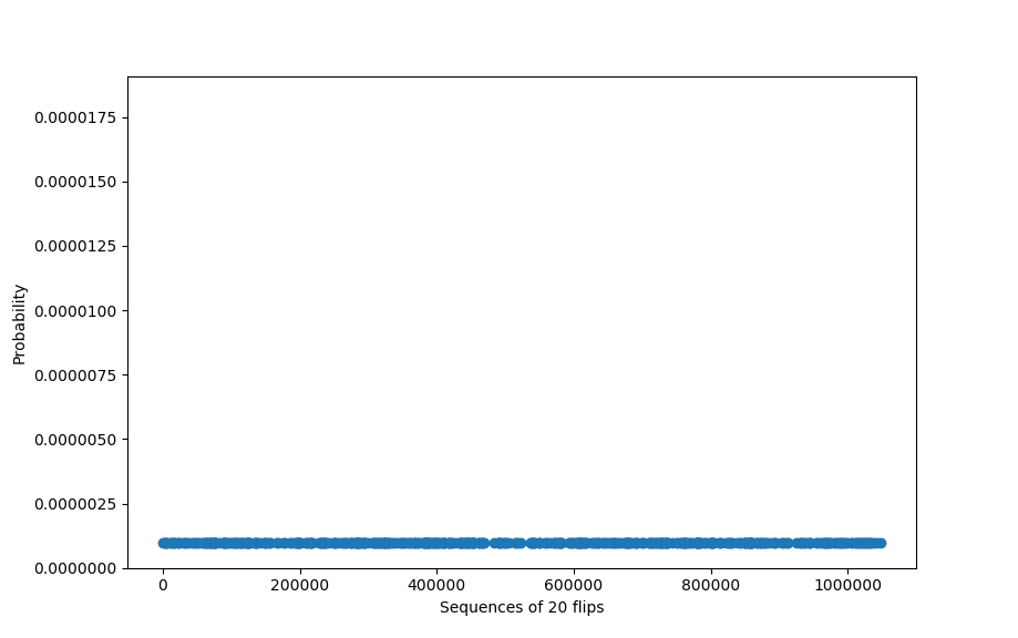
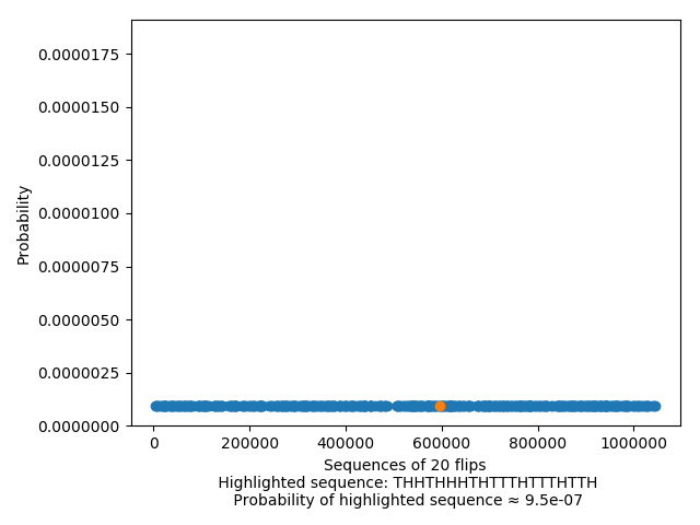
And looking at the chance of any one sequence is just looking at the (tiny, tiny) value of any one of these points:

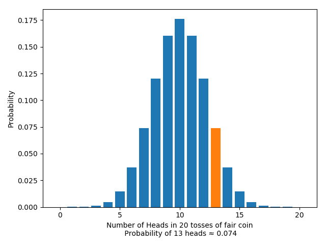
On the other hand, if we look at the distribution of the chosen test statistic, the number of heads, we get the binomial distribution we derived above:

Looking at the likelihood of the test statistic itself amounts to just looking at the likelihood of getting some particular number $m$ of heads:

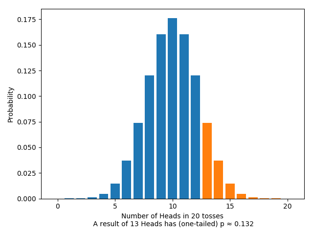
On the other hand, looking at the $p$-value means looking at the likelihood of getting any result as or more extreme than $m$ heads: rather than one single result, we’re looking at the area of an entire region. For the one-tailed test, this looks like:

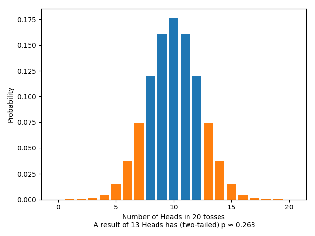
And for the two-tailed test, this looks like:

The General Procedure: A Warning

Let’s go over the driving idea behind the test. We want to test whether your coin is fair. Assume for a moment that it is fair. Then if we flip it 20 times, we expect to get about 10 heads. Suppose we actually get 8 heads. That’s not surprising, given our assumption. After all, we only expected to get about 10 heads, not exactly 10 heads. So the result doesn’t call our assumption into question. Suppose instead we actually get 4 heads. To get a result that far from 10 is surprising, given our assumption. So the result does call our assumption into question: either a surprising thing happened or our assumption is wrong. Now, surprising things do happen, but they don’t happen that often, else they wouldn’t be surprising. So the better bet is to reject the hypothesis that the coin is fair. That’s the idea behind significance tests.

In general, suppose we wish to test some probabilistic hypothesis, designated the null hypothesis. Design an experiment and determine all possible experimental outcomes. Then choose a test statistic, which associates a number with each outcome. Assuming that the null hypothesis is true, work out the distribution of the test statistic: that is, for each possible value of the test statistic, work out the probability of getting that value. Next, choose a significance level $\alpha$, typically 0.05 or 0.01, and decide whether to do a one-tailed or two-tailed test. Then do the experiment and note the actual value of the test statistic. Work out the the $p$-value. If the $p$-value is less than $\alpha$, reject the null; else, don’t.

Life would be much easier if the $p$-value of an experiment were the probability that the null hypothesis is true. But it’s not. The truth is more of a mouthful: the $p$-value is the probability of getting a value for the test statistic at least as extreme as the actual value, assuming the null is true. That is quite different to the probability that the null is true.

A lot of technical work has gone into developing significance tests. For example: working out the distribution of a test statistic can be hard and require some sophisticated math; extending the tests to cases where the data is continuous requires further machinery. But the driving idea behind significance tests is simple: do an experiment, and check how extreme the result is, assuming the null.

A different experiment

Suppose we had done our experiment differently: instead of flipping a fixed number of times, we decide we’ll keep flipping until we get a total of 6 tails. This is a perfectly sensible test, because we expect different behaviors from a biased coin and a fair coin: we’d expect a fair coin to take around 12 flips to get 6 tails, a tails-biased coin to do so in fewer flips, and a heads-biased coin to take a longer number of flips. We can even keep the same test statistic: the number of heads will vary between runs, since the length of runs will vary, and the number of heads is always 6 less than the number of flips. We expect around 6 heads for a fair coin. But in this setup, the distribution of the test statistic is different.

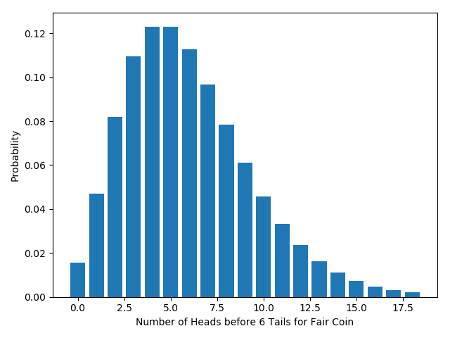
What is the distribution? We can work this out from the principles above. Assume the coin has a probability $q$ of getting heads on each flip. If a complete run of our experiments results in $m$ heads, we must have flipped it $m+6$ times, with tails on the final flip. In other words, we get a total of $m$ heads if and only if we got $m$ heads in the first $m+5$ flips, and then a tail. The chance of getting $m$ heads in the first $m+5$ flips is given by the binomial distribution we derived early on: ${m+5 \choose m} (1-q)^5 q^m$. The chance of getting a tail on the final flip is just $1-q$. So the total probability of getting $m$ heads is just ${m+5 \choose m}q^m (1-q)^6$. More generally, the total probability of getting $m$ heads by the time we get $r$ tails is ${m+r -1 \choose m} q^m (1-q)^r.$

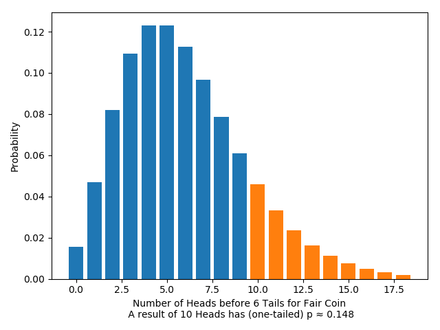
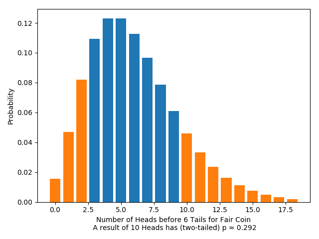
Again, this distribution has a special name: the “negative binomial distribution”. If we graph this distribution for a fair coin ($q=0.5$), it looks like this:

As before, we can calculate the $p$-values (one- and two-tailed) for any given result. For example:

Significance tests are sensitive to the stopping rule

We can express the difference between the two experiments as a difference in when we agree to stop the experiment. In the fixed-number-of-flips experiment, we stop when and only when we reach our target number of flips. In the fixed-number-of-tails experiment, we stop when and only when we reach our target number of tails. In other words, the two experiments have different stopping rules. (Of course, innumerably many other stopping rules are possible too.)

Suppose we perform both experiments: in the fixed-flips experiment we decide to flip a total of 20 times; in the fixed-tails experiment, we decide to flip until we get 6 tails.

Some outcomes are possible in your experiment but not mine, such as a sequence of 9 h‘s and 11 t‘s; other outcomes are possible in mine but not yours, such as a sequence of 8 h‘s and 6 t‘s, ending in a t; but some outcomes are possible in both our experiments, such as hhhththhhhhthhthhhtt, a total of 6 tails, 14 heads.

Let’s do significance tests on the two experiments. As far as our choices of conventions, we’ll pick the same conventions for both: both will test the null hypothesis that the coin is fair; both will use the number of heads as a test statistic; both will use a two-sided test; both will reject the null hypothesis only if the $p$-value is less than $0.05$ (a typical choice). Let’s suppose that, as it happens, we get the same outcome in both experiments, the one at the end of the previous paragraph.

Pulling from the above, for the fixed-flips test we have:

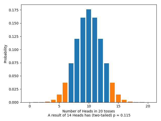
The $p$-value here is greater than $0.05$: according to the test, it’s not a result significant enough to warrant rejecting the null hypothesis that the coin is fair.

At the same time, for the fixed-tails test, we have:

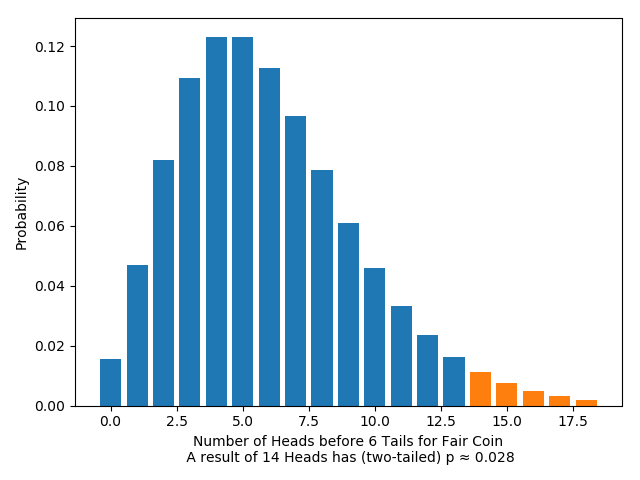
The $p$-value here is less than $0.05$; according to the significance test, this is a result that is significant enough to warrant rejecting the null hypothesis.

But the only difference between the two situations is the stopping rule used! In other words, the very same sequence of coin flips, with the very same conventions, leads to opposite conclusions, depending on which stopping rule was used. That’s what we mean when we say that significance tests are sensitive to the stopping rule.

Is sensitivity to the stopping rule a problem for significance testing?

Plenty of other objections have been leveled at significance tests. But sensitivity to the stopping rule is at the heart of the dispute. Take Deborah Mayo, for example, a staunch defender of significance tests: “Edwards, Lindman, and Savage, quite rightly, regard this difference in attitude on the relevance of stopping rules as a central point of incompatibility between [rival methodologies in statistics].” (Mayo, 1996: 342) Howson and Urbach agree on the centrality of stopping rule sensitivity, although they disagree with Mayo about what conclusion we should draw from it: “The fact that significance tests [are sensitive to the stopping rule] is a decisive objection to the whole approach.” (Howson and Urbach, 2006: 159)

So, then, is sensitivity to the stopping rule a problem for significance testing or not? Examples involving coins can make the question seem academic. Far from it: if stopping rule sensitivity is a problem, we need to know. The question isn’t academic, and nor is it easy. The rest of the post sketches some of the arguments, pro and con. The parts can be read in any order. About half of what I write below is false. But which half?

Irrelevance.

Cheating

Suppose you are an unscrupulous scientist, seeking reason to reject some rival scientist’s hypothesis. Perhaps you can exploit sensitivity to the stopping rule: do a significance test, choosing your stopping rule carefully so as to boost the probability of rejecting the hypothesis.
$$$$
Take your coin. Suppose I offer a prize if you manage to bias it; I’ll award you the prize if a two-tailed significance test, with test statistic the number of heads, rejects the hypothesis that the coin is fair at a significance level of 5%. You could just do a fixed-flips test, flipping it 20 times, say. But how might you exploit sensitivity to the stopping rule to boost your chances of rejecting the null and winning the prize?
$$$$
Here’s one attempt: flip the coin until you have 10 more heads than tails. Actually, let’s add a cut-off: flip the coin until you have 10 more heads than tails *or* you’ve flipped it a total of 100 times, whichever comes first. (Adding the cut-off simplifies the analysis; but we could make the same point even if we dropped it.) Call this the *fixed-difference* stopping rule. By choosing the fixed-difference rule, you’ve considerably boosted the probability that you’ll get 10 more heads than tails. So haven’t you also boosted your chances of rejecting the null?
$$$$
Let’s work it through. First, take the fixed-flips test. When will we reject the null? Well, if we observe no heads at all, we’ll get a *tiny* $p$-value ($2 \cdot \frac{1}{2^{20}}$), so reject. If we observe 1 head, we’ll get a slightly bigger, but still tiny, $p$-value, and still reject. Calculating $p$-values in turn for each possible number of heads, it turns out we reject if the number of heads is between 0 and 5 or 15 and 20, inclusive. So the probability that we reject is the probability that we get between 0 and 5 heads or 15 and 20 heads, inclusive. Assuming the null is true, that’s about 4.1%.
$$$$
What about the fixed-difference test? This is more complicated. In the fixed-flips test, we can get any number of heads from 0 to 20; but in the fixed-difference test, we can get any number of heads from 0 to 55. (Exercise: Why can’t we get more than 55 heads?) To derive the distribution takes some work (if you’re interested, google “simple random walk”), but here’s the graph:

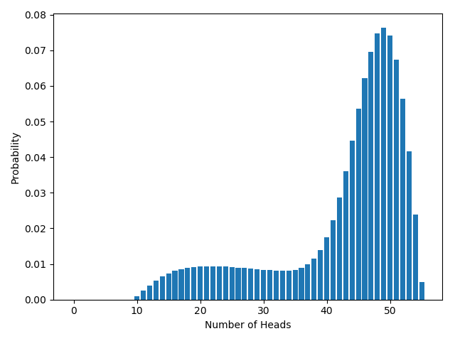
When will we reject the null? Calculating $p$-values in turn for each possible number of heads, as before, it turns out we reject if the number of heads is between 0 and 17, inclusive. So the *probability* that we reject is the *probability* that we get between 0 and 17 heads, inclusive. Assuming the null is true, that’s about 4.3%.
$$$$
So, admittedly, with the fixed-difference rule we have a slightly higher chance of rejection than with the fixed-flips rule. But the difference is small (4.3% v. 4.1%). That sort of fluctuation isn’t surprising. For example, the chance of rejection in a fixed-flips test where you flip it 20 times is slightly different to the chance of rejection in a fixed-flips test where you flip it 30 times, which is slightly different again to the chance of rejection in a fixed-flips test where you flip it 40 times. Whenever you change your stopping rule, a small fluctuation in the chance of rejection is to be expected. The key point is that when you moved from fixed-flips to fixed-difference, the chance of rejection was pretty much the same; you certainly didn’t significantly boost your chance of rejecting the null, as you hoped.
$$$$
There’s no deep mystery here. When we moved from fixed-flips to fixed-difference, we *did* boost the chance of observing 10 more heads than tails; in the fixed-flips test, observing 10 more heads than tails (i.e. 15 heads and 5 tails) leads us to reject the null. *but in the fixed-difference test, it doesn’t.* Why not? Because changing the stopping rule also changes the distribution of the test statistic, and so changes which values for the test statistic lead to rejection. What you’ve gained on the swings, you’ve lost on the roundabouts. In fact, it’s straightforward to show that in any significance test, the chance of rejection, assuming the null, is at most the significance level. Change the stopping rule however you like, you won’t boost the chance of rejection above 5%.

Rarity

Probability of false rejection

Relevance

Stopping rules in practice