Hysteresis & Student Debt

The geographic character of the Great Recession of 2008–2009 is, by this point, well-known. While everywhere in the United States experienced a sharp increase in unemployment, some areas suffered disproportionate exposure to subprime mortgages and the consequent bursting of the housing bubble, and some experienced the cyclical downturn more harshly than others, with larger shares of local employment in harder-hit industries.

The Great Recession is also substantially at fault for the student debt crisis, and the geographic contours of the downturn carry implications for how student debt has been experienced throughout the country. The number of borrowers and average loan balances were increasing rapidly before the onset of the financial crisis, thanks to the defunding of public university systems following the previous cyclical downturn in the early 2000s. The Great Recession put those trends into overdrive: with fewer jobs available and a more selective labor market, many young people were funneled into a higher education system already in the process of becoming much more dependent on students and their families paying hefty tuition, as opposed to state support. Those who had entered the system seeking credentials to boost their job prospects then graduated (or didn’t graduate) into a labor market still suffering from stagnant wages and disappearing job opportunities. Credentialization cascaded into higher loan balances as a share of income, rising delinquency, and eventually declining repayment rates.

Our research is the first, to our knowledge, to examine the Great Recession and the student debt crisis together at an individual, as opposed to macro, level. Our starting point is the economics literature that links exposure to the Great Recession to prolonged labor market distress lasting years after the Great Recession was formally over. Economic growth resumed by 2010, but the downturn’s negative effect on employment and earnings for those most affected lasted at least through the mid-2010s, and most likely through the present. This phenomenon is known as “hysteresis” in the labor economics and macro literature, drawing on the physics concept that refers to the path-dependence of outcomes in response to a transitory shock. The paper in that literature that most directly inspires the approach we take is Yagan (2019) “Employment Hysteresis from the Great Recession,” which finds that a local area unemployment rate increase during 2007–2009 caused lasting reductions in employment and earnings for individuals, regardless of whether they were unemployed during that period. Specifically, the paper estimated that a one-percentage-point unemployment rate increase was associated with a reduction in the probability of being employed in 2015 of 0.393 percentage points and a reduction in annual earnings of $997.

In this study, we consider the Great Recession’s effect on student debt–related outcomes, extending the logic of papers like Yagan’s to the student debt crisis, given the apparent relationship between labor market distress and prolonged enrollment in higher education, rising tuition, institutional segregation, earnings insufficient to pay off loans, and all the many other ways in which the student debt crisis is one facet of overall dysfunction in the labor market. We find that where a person lived during the Great Recession affected not only their employment outcomes, but also their student loan balances, eventually resulting in an accumulating burden of unpaid debt amidst a still-slackened labor market. Using a specification constructed to be as similar as possible to Yagan (2019), we show that an increase of one percentage point in the local area unemployment rate between 2007–2009 is associated with an increase in student loan balances of around $812 by 2019, an increase in required monthly payments on student loans of $5.10, and a reduction in the probability of having fully repaid outstanding student loans by 2019 of about 0.75 percentage points. These effect sizes are large, the more so because the Great Recession shock was severe: the median level of the shock is approximately 4.5 percentage points. Thus, our estimates imply that someone subjected to the median shock would have a student loan balance over $3500 higher than they would have had the Great Recession not occurred. Moreover, we find larger increases in loan balances for the younger cohorts of borrowers within our overall sample of borrowers aged 18–34 in 2009, suggesting that the effect of the Great Recession on the student debt crisis was even worse for those who were not yet old enough to have taken on student debt in 2009.

Data

The basis for our study is a panel dataset of the credit reports of one million student borrowers starting in 2009 and lasting a decade, until 2019. The sample frame is that an individual had to be between the ages of 18 and 34 in 2009 and have an outstanding student loan balance at that time.¹ We observe some demographic characteristics directly in the sample, including age, gender, and several geographic variables derived from the individual’s address.

We further observe individual-level, credit-relevant outcomes separately for each year. For the purpose of this study, we focus on student debt–related outcomes: total balance on all outstanding student loans, total monthly payments on outstanding student loans, and a variable we constructed to encode whether an individual who had outstanding student debt in 2009 had paid off all their student loans by the relevant subsequent year. We construct this last outcome by observing the succession of outstanding balances: if an individual has declining total balances year-by-year, and reaches a balance of zero on their outstanding loans by a given year, we code that person as having fully repaid their loans in that year. Provided we don’t observe a subsequent positive balance, we assume that that remains the case going forward. Previous work in this series has documented repayment among this cohort of student borrowers: the median borrower still had approximately 37 percent of his or her 2009 balance outstanding in 2019, and over 25 percent of borrowers had more student debt outstanding in 2019 than they did in 2009.

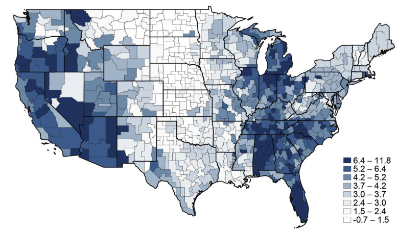
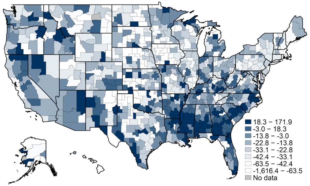
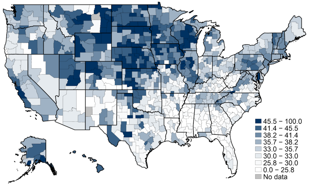
The premise of this study is that the geographic area in which someone lived during the Great Recession is a proxy for how severely they were affected by the Great Recession, similar to the study by Yagan. It thus uses the change in unemployment rate between 2007 and 2009 in the commuting zone where an individual lived in 2009, the first year of our data, as an index for how “shocked” that individual was by the Great Recession. Commuting-zone-level changes in unemployment rates are available from Professor Yagan’s replication files for his 2019 paper, constructed from county-level unemployment rates in the Bureau of Labor Statistics’s Local Area Unemployment Statistics and mapped in Figure 1.

Regression equation

The main regression specification is of the form:

\begin{equation} y_{i,201t} – y_{i,2009} = \alpha + \beta SHOCK_{c,2007-2009} + \gamma x_{i, 2009} + \delta x_{i, 201t} + \epsilon_{i, 201t} \end{equation}

where i indexes an individual in the panel data, c refers to the local area (commuting zone) in which that individual resided in 2009, and t refers to one of the “outcome” years 2010–2019. In this instance, SHOCK refers to the percentage point change in the commuting zone unemployment rate between 2007 and 2009, in line with Yagan (2019). The regressors x refer to individual-level covariates, separated into those observed for an individual in 2009 and those observed in the outcome year 201t. The outcome of interest y is expressed as the difference in that outcome in 201t relative to the baseline year 2009. ε is an individual-year disturbance term assumed to be uncorrelated with the value of the shock.

The coefficient of interest in this regression is β, which is interpreted as the causal effect of a one-percentage-point higher value of the shock (i.e, an increase in the unemployment rate of one percentage point between 2007 and 2009 in the commuting zone in which individual i lived in 2009) on the outcome of interest, denominated in units of the outcome of interest.

Covariates include age, gender, student loan balance in 2009, and the contemporaneous unemployment rate in the commuting zone in which individual i resides in the regression outcome year (which need not be the same commuting zone as in 2009). Everyone in the panel was a student debtor, at least in 2009. The controls seek to isolate the effect of the Great Recession among individuals in that broad group, i.e. comparing individuals of the same age, gender, and outstanding student loan balance in 2009. The idea is that individuals in the overall sample may be at very different places in their educational attainment or economic life cycle, and we want to compare otherwise-similar individuals depending on how affected they were by the Great Recession to ascertain the effect of the Great Recession on student-debt-related outcomes. The identifying assumption is that conditional on those covariates, differences in outcomes between individuals (with the same age, gender, and student loan balance in 2009) that emerge subsequent to 2009 are caused by differences in the severity of the Great Recession shock.

Results

As stated above, we focus on three student debt–related outcomes of interest: total student loan balance at the individual level, total required monthly payments on student loans, and whether an individual completed repayment on all outstanding student loans. For each of those outcomes, we report the regression results for each year after 2009. All outcomes are defined relative to a 2009 baseline, given that all individuals in the sample had student debt outstanding in that year. The first two outcomes of interest are a dollar change since 2009, while the “completed repayment” outcome is binary.

Table 1 reports the regression of change in student loan balance between 2009 and 2019 on the shock and covariates. The preferred specification is given in column 5, with all covariates added. The point estimate 812.2 signifies that a one-percentage-point-higher unemployment rate change between 2007 and 2009 corresponds to an increase in outstanding balance between 2009 and 2019 of \$812.20. All regressions utilize robust standard errors clustered at the level of the commuting zone of residence in 2009.

It’s also worth noting some of the patterns in estimated coefficients on the covariates: women appear to take on more student debt than men and, given this is a sample of student debtors aged between 18 and 34 in 2009, younger borrowers in that sample end up taking on more student debt subsequent to 2009 than older borrowers. Probably for related reasons, borrowers who had more student debt already outstanding in 2009 subsequently took on less. These two facts highlight life cycle heterogeneity present in the sample. Borrowers who lived in areas with higher unemployment rates after 2009 also took on more debt.

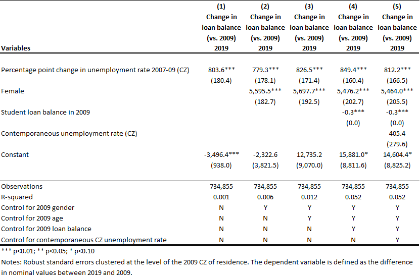
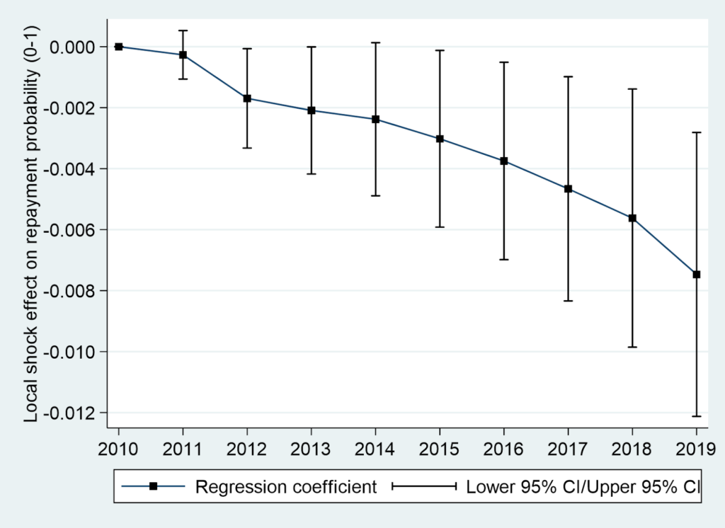
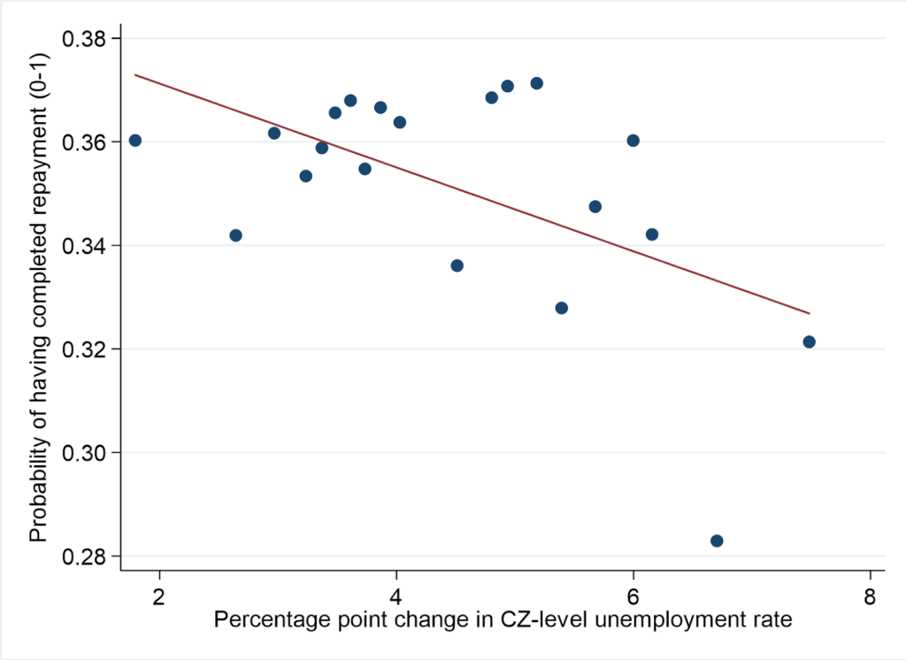
Figure 2 visualizes these results in two different ways: first, by running the regression separately in each year from 2010–2019, it shows an increasing effect of the Great Recession shock, suggesting that the effects are not dissipating over time, but rather the opposite. Second, for the outcome year 2019, the binned scatterplot depicts ventiles of the shock on the horizontal axis. The vertical axis plots the average value for the outcome within that shock ventile (net of the same controls used in column 5 of regression Table 1). The best-fit line plots the estimated relationship, and thus its slope is approximately equal to the regression coefficient of 812.2. Note that the domain for the shock is between just under two percentage points for the least-shocked 5 percent of commuting zones (i.e., their unemployment rate rose by slightly less than two percentage points) and over seven percentage points for the most-shocked 5 percent. Negative numbers on the vertical axis represent declining average student loan balances between 2009 and 2019, and positive numbers represent increasing balances.

Thus, altogether the takeaway from Figure 2 is that student debtors who lived in the most-shocked commuting zones experienced rising student loan balances between 2009 and 2019, and people who lived in the least-shocked commuting zones experienced declining balances, with the gap between them widening over time.

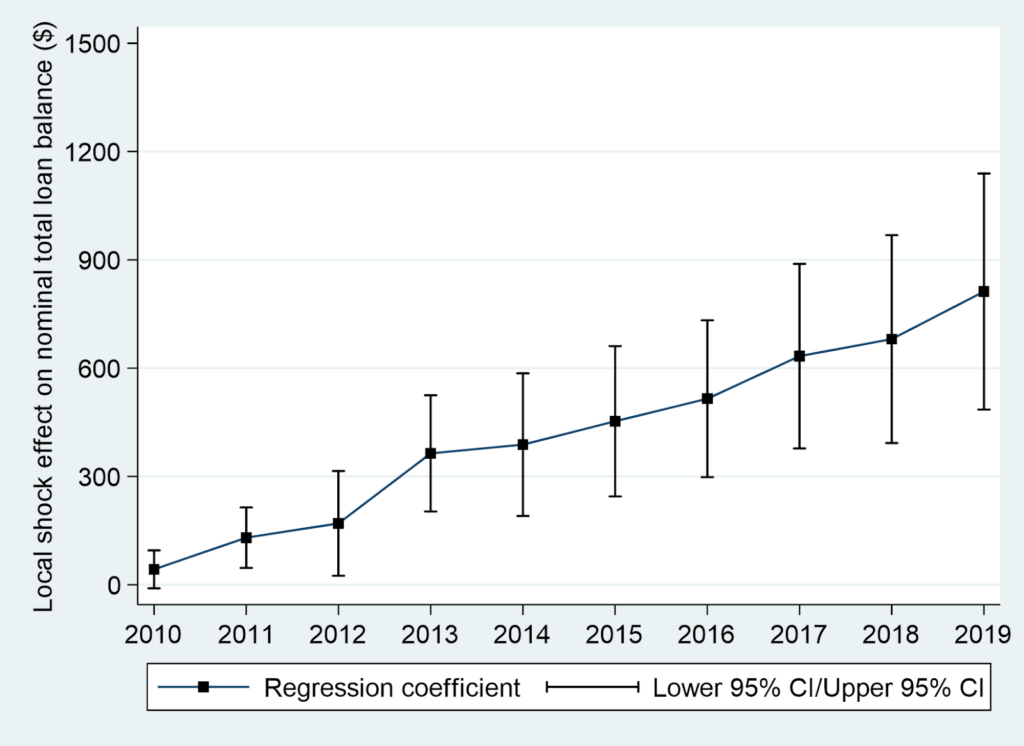
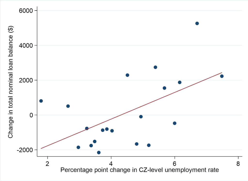
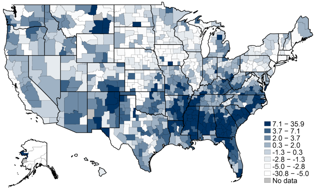
Table 2 reports the same regression specifications as in Table 1, but with the change in total monthly payments on student loans between 2009 and 2019 as the outcome of interest, rather than the change in total outstanding balance. Here the point estimate in the preferred specification is 5.1, meaning that a one-percentage-point-higher change in the unemployment rate in 2007–2009 corresponds to a $5.10 higher student loan payment in 2019 relative to 2009. Figure 4 consists of the same two plots as in Figure 2, for this additional outcome of interest.

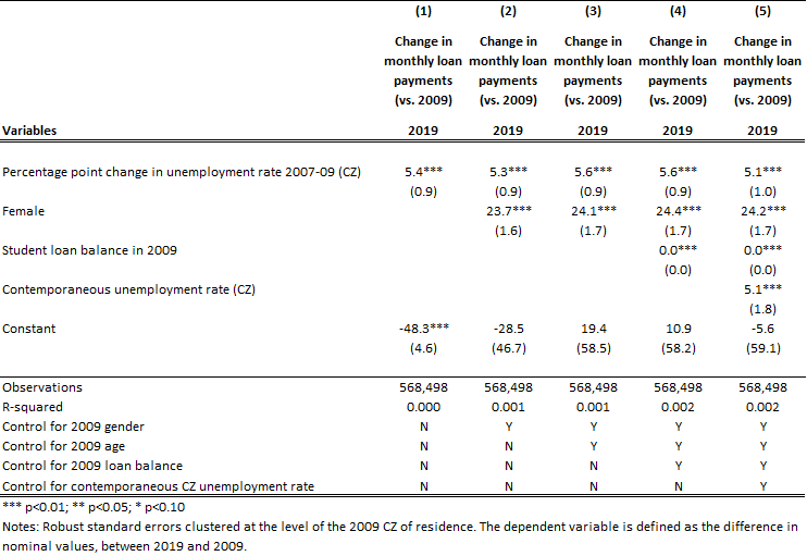
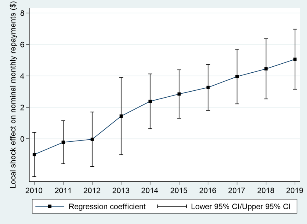
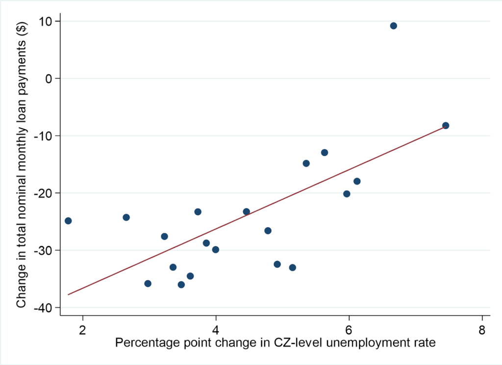
There are several things to note about this second monthly payments outcome: first, it appears to be a lagging indicator, relative to total student loan balance, likely because of the deferment that student debtors enjoy for the time following the issuance of their loans if they remain enrolled, and (usually) for six months following graduation. Hence required payment amounts lag loan balances, and the Great Recession effect does not emerge until 2013 or 2014, whereas it appears in 2010 for outstanding balances. Second, for the change in monthly payments outcome, almost all ventiles of the shock variable show declining payments between 2009 and 2019, but the decline is smallest in the most shocked. This likely relates to two things: increased enrollment in income-driven repayment after 2016, resulting in lower payment amounts relative to income but also reduced repayment of outstanding balances. That means that required payments last longer, and (consequently) a smaller share of borrowers in the most-shocked commuting zones reach full repayment by the end of the sample.

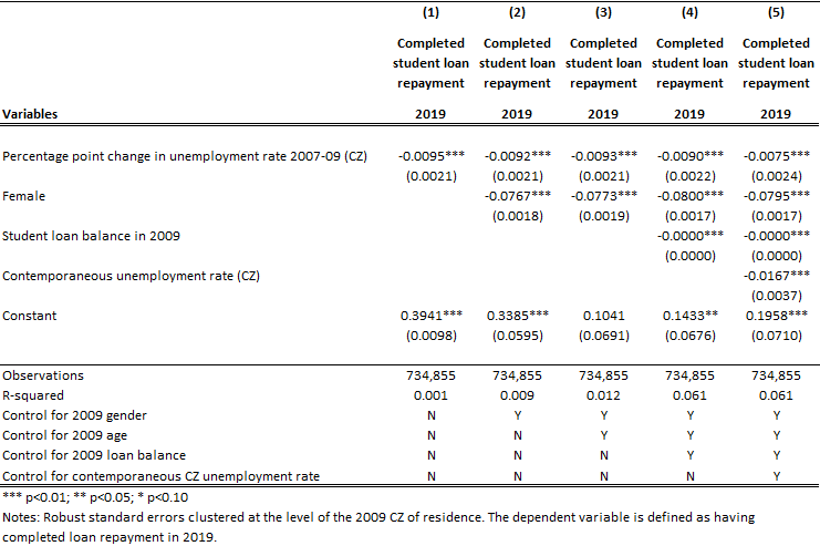
Table 3 focuses on this last outcome of interest: likelihood of full repayment. Note again that this outcome is specified in levels, i.e. a binary outcome for completed repayment, and not a difference relative to 2009 (since everyone in the sample had outstanding student debt in 2009). The regression table indicates that a one percentage point-higher unemployment rate change between 2007 and 2009 corresponds to a 0.75-percentage-point-lower probability of full repayment in 2019. The effect of the shock on full repayment also amplifies over time, as with the previous two outcomes.

Threats to identification

Relative to the estimation strategy on which this study is based, the one adopted in Yagan (2019), this study has two shortcomings, one minor and one more significant. First, we only start to observe the individuals in the panel in 2009, at the end of the Great Recession shock interval rather than the beginning, and we observe fewer (and likely less reliable) demographic and economic covariates in the credit reporting data (age, gender, and “starting” student loan balance) than in the previous study’s tax return data (age, pre-recession earnings, and pre-recession industry of employment). In that sense, there is probably more residual variation in the population net of controls in our study than in Yagan’s, when the design seeks to create as homogeneous a sample as possible that differs only in the extent to which it is affected by the Great Recession (although it should be noted that our sample is inherently more homogeneous in age and the fact that they’re all student loan borrowers). We view these deficiencies as minor, however, since variation in terms of when someone was affected matters less than the degree to which they were affected. Yagan (2019) shows some variation along these lines, for example among the subsample subjected to mass layoffs (who experienced the shock of the Recession earlier) and the subsample who worked in national retail chains (for whom the effect took longer to materialize).² Notwithstanding those differences, though, the timing for the Great Recession effect on both employment and earnings in both subsamples was qualitatively similar in the following years 2010–2015.

The bigger threat to identification is that we do not observe any of our student debt–related outcomes prior to 2009, which means that we cannot directly reject pre-trends in those outcomes among individuals who lived in commuting zones that were differentially affected by the Great Recession. The problem with our inference would arise if the commuting zones most severely impacted by the Great Recession were those in which the student debt crisis had been getting worse before 2007, relative to the commuting zones less affected by the Great Recession. That would mean that the effect we attribute to the Great Recession’s severity might in fact be caused by something else, violating the identification assumption that the error term in the regression equation is uncorrelated with the shock regressor. Note that this is relevant for differences in trends, not levels: it doesn’t matter if the commuting zones most affected by the Great Recession were also already those most affected by the student debt crisis: the regressor of individual-level 2009 student loan balance should account for that level effect. What would undermine the inference is if balances were rising faster in the most-affected commuting zones, versus the less-affected ones, prior to the onset of the Great Recession.

We nonetheless feel fairly confident in placing a causal interpretation on our Great-Recession-related shock’s effect on student debt outcomes. There is substantial geographic variation in the severity of the student debt crisis, but that variation is driven mostly by state-level policy variation—the degree to which public higher education systems depend on public funding versus tuition, as well as geographic variation in different types of institutions with varied business models. (For example, living near for-profit institutions correlates to increased student loan balances and other pathologies of student debt.) These things are not closely related to the severity of the Great Recession shock, at least not prior to the Great Recession. It is likely that the Great Recession may have caused states to disinvest from public higher education and allowed for-profit institutions to enter and expand in areas that suffered severe labor market distress, but these responses would have happened during and after the Great Recession. Thus these mechanisms are some of the many that are properly understood as giving rise to the causal relationship(s) we estimate.

Finally, Yagan (2019) is able to test for pre-trends and rejects them in relation to the outcomes that the paper focuses on: employment and earnings. It would be surprising, then, if there were pre-trends in our student-debt-related outcomes, less closely related to the causes of geographic variation in the Great Recession’s effects, but not in outcomes that are more closely related to the variation that manifested during the Great Recession. We also include the contemporaneous unemployment rate in our regression specifications to try to control for possible proxies for geographic variation in long-term student-debt-related outcomes and also with the Great Recession shock itself.

Interpretation

The Great Recession was undoubtedly a major impetus for the student debt crisis: college enrollment increased, student loan levels shot up, young workers in particular had trouble accessing full-time employment early in their careers and thus remained in education longer, at the same time as student-facing costs were rapidly increasing due to state disinvestment. As time went on, increased loan amounts, particularly among so called non-traditional populations, caused rising delinquency and default on student loans, giving way to rising enrollment in Income-Driven Repayment by the late 2010s, resulting in lower repayment. That broad narrative is well-known, though this study is the first to have documented it in individual-level panel data. Doing so demonstrates that student debt represents one facet of poor labor market functioning in younger cohorts entering the labor market in the aftermath of the Great Recession. Yagan (2019) highlights the exit-to-nonemployment channel for the employment effects documented in that paper, and one possible nonemployed labor market state may be enrollment in higher education, resulting in rising student indebtedness.

The ostensible purpose of taking out student loans to finance higher education is that it is an “investment” that “pays off” in the form of higher earnings and more secure employment for higher-skill workers. That idea has motivated policies that ushered in the student debt crisis, such as rising maximum loan levels and the proliferation of accredited degree programs, and implies that those with student debt must be better-off than those without, since they also have more education and thus more skills, resulting in higher earnings. The inference of this study is the opposite—student debt signifies worse luck in the labor market, in the sense that it’s associated with having experienced a more severe Great Recession shock, which has lasting effects in terms of worsening labor market outcomes. These results therefore strongly contrast with the view that there’s nothing significantly wrong with rising student loan balances and the resulting non-repayment of outstanding loans because student borrowers “do well in the labor market” and are privileged relative to the rest of the population.

Modestino, Shoag, and Ballance (2019) show that during the Great Recession, when labor markets were slack and employers were able to be selective about which workers they hired, job ads specified higher education, experience, and skill levels for a given job title. That effect trailed off as the recovery from the Great Recession played out, but the basic insight of that research is that the “skills” required of a given job are not (entirely) intrinsic to that job, but rather determined by slackness in the labor market shifting greater bargaining power to individual employers. It’s not hard to imagine this dynamic driving a response from workers to seek credentials (or “skills”), and thus take on more student debt. If education and the debt required to obtain it doesn’t correspond to higher salaries, then, it’s not surprising that they’d have more trouble paying it off.

Moreover, the panel this study utilizes consists of people who already had student debt in 2009, and we show that the effect of the Great Recession on student debt accumulates over time for that group. Given that pattern, there are probably more dire effects of the Great Recession shock on younger cohorts that did not yet have student debt in 2009 but who entered labor markets seemingly permanently slackened by the effect of the Great Recession. The literature on the Great Recession’s effect on job ladders and economic life cycles tends to focus on people who were in the labor market during the Great Recession, and it implies that that group is permanently, but anomalously, worse-off than cohorts both preceding and succeeding it. It may be that subsequent cohorts are in fact even worse off. The fact that the youngest borrowers present in our panel tended to take on the most debt between 2009–2019 points in the same direction. Student loan repayment across cohorts is undoubtedly getting worse over time, and that trend persisted despite the relatively healthier labor market of the late 2010s, prior to the Covid-19 recession. All of that suggests that subsequent cohorts of borrowers would be worse off relative to the cohort studied here.

A major outstanding question from this study relates to the precise interpretation of the Great Recession shock, and the resulting hysteresis, in labor economics terms. Did the recession represent a decline in labor demand against a more-or-less constant labor supply curve, or did the resulting power shift in the labor market mean that workers became less wage-elastic vis a vis individual employers due to the paucity of outside job opportunities, and thus better able to be exploited? In reality, the answer is probably both, but interpretation of the various mechanisms awaits further work that is able to distinguish between these two causes.